
TFQA: Tools for Quantitative Archaeology
kintigh@tfqa.com +1 (505)
395-7979
TFQA Home
TFQA Documentation
TFQA Orders
Kintigh(ASU
Directory)
|
TFQA: Tools for Quantitative Archaeology |
TFQA Home |
Rarefy: Rarefaction Diversity AnalysisPerforms rarefaction analysis for sets of sample counts in a CSV file, as described by Baxter (2001). Provides expected richness, the standard deviation of the expected richness as well as the Z score and probability for each larger sample rarefied to every smaller sample size. Also outputs expected richness for each sample up to its sample size for graphing. (An additional program, Rarefy_1.exe, is provided if you wish to get results on the rarefaction of only a single sample. That program is not separately documented but the operation should be self-evident.) Rarefy is a Windows program written in Delphi, an extension of Pascal as implemented in the Embarcadero RAD Studio XE. Running the program Important information on TFQA programs may be found at https://tfqa.com. See especially, Program Conventions and Running TFQA under Windows. To run the program, copy Rarefy.exe to a directory that includes the input data files you wish to evaluate (in CSV Format, as described below). Having navigated to that folder, when you double click on Rarefy.exe the program opens a Windows "Run" Window . The program will prompt you for information that it needs to run. Default answers are provided in {curly braces} and can be obtained by just pressing Enter. Reply Y or N to yes or no questions. Sample Input file (conkey.csv) The program looks for input in a .csv file. Each case is represented by a single line with a set of counts for the different classes. The first line of the file can be a set of column labels separated by commas (as normally interpreted in CSV files), or the first line can start with the counts. If there is no label line, the program will simply use sequential input case numbers. Case or variable labels with embedded blanks or special characters must be enclosed in quotes (e.g., "variable name"). All numeric variables are assumed to be counts. The sample input file reproduced below is abbreviated, as indicated by the ... ellipsis. Rarification of a given sample provides expected richness values for smaller sample sizes. Usually, the observed distribution of counts of a larger sample is used to generate expectations for all smaller sample sizes. However, in some cases, it may also make sense to generate expectations from either the the combined counts of all observed samples or from a hypothetical sample with (large) counts dictated by a theoretical distribution. In these latter cases, once can just add one or more observations to the input data set with the desired sets of counts. These additional observations will not affect the program's calculation of expectations between observed samples. However, if an MDS is performed, the combined sample will affect the results. Site,V1,V2,V3,V4,V5,...,V57 Alta/Altamira,2,12,7,1,0,...0 "Mina/Cueto de la Mina",1,12,2,0,1,...,0 "Cier/El Cierro",0,5,1,2,0,...,0 "Juyo/El Juyo",0,8,2,1,0,0,...,0 "Palo/La Paloma",0,4,0,0,0,...,0Sequence of Program Prompts +------------------------------------------+
¦ Rarefy V3.0 ¦
¦ Compute Rarefaction Diversity Statistics ¦
¦ ¦
¦ (C) 1986-2020 Keith W. Kintigh ¦
¦ All Rights Reserved ¦
¦ ¦
¦ 421 Calle Kokopelli ¦
¦ Santa Fe, NM 87501 ¦
+------------------------------------------+
File of Input Frequencies {.CSV} ? conkey
File: CONKEY.CSV
First line interpreted as labels for 58 variables:
5 obs & 58 vars; 57 numeric & 1 string
File Variables:
1"Site 2=V1 3=V2 4=V3 5=V4 6=V5 7=V6 8=V7
9=V8 10=V9 11=V10 12=V11 13=V12 14=V13 15=V14 16=V15
...
57=V56 58=V57
Variable Number of Default Case Label (Reply 0 for case Number) {0} ? 1
The program asks for the input file name and reports the number of observations and variables and the variable labels (generated if none are provided). The program then asks which variable should be used as a case label. Other non-numeric variables are ignored. Note: Sample Sizes Range from 23 to 152 Total: 332 Note: Richnesses Range from 12 to 38 Report on the program input. Printed Analysis Output File (CON for console) {CONKEY.TXT} ?
File Exists; OK to Erase It {N} ? y
CONKEY.TXT Erased
Analysis Title for Output ? Conkey: Engraved Bone Designs
Output Line Width (in characters) {120} ? 90
Print Length for Observation Labels {12} ? 4
Print Z Score and Probability Matrices in [T]riangular or [S]quare Form {S} ?
Number of Decimals in Printed Output {3} ?
Print Input Data Set (Sorted by Sample Size) {Y} ?
The program then asks a series of questions about the output: the output file name, descriptive title, line length (triangular matrices will be easier to read with longer line lengths), the number of characters to use in the printed observation labels, and the number of decimals printed. The label variable in the input dataset may have, long, descriptive labels for the observations. However, only the specified number of leading characters will be printed. Thus, the label value "Palo/La Paloma" will be printed only as "Palo" if 4 characters is specified as the printed length of the observation labels. The maximum length that can be printed for an observation label is 12. The program also asks if you would like the distance matrix output in (lower) triangular or square form and if you would like the input data printed to the output file. Phase 1 Computation Begins 100% Complete Phase 1 Computation Ends Phase 1 Compute Time: 0.0 Seconds Report on the program progress. Write Triangular Matrix of Probabilities for Analysis in R {Y} ? y
Output File for Distance Matrix {CONKEY.DST} ?
File Exists; OK to Erase It {N} ? y
CONKEY.DST Erased
The program asks if you would like the output probability matrix saved in a file for additional analysis (e.g. via multidimensional scaling in R). Write Expected Richness Values for SS of 1 to N for Each Case {Y} ?
Output File for Distance Matrix {CONKEY_P.CSV} ?
Maximum Sample Size Plotted {69} ?
Finally the program asks if you would like to calculate and save the expected richness and standard deviations for each case, for sample sizes of 1 to the sample size of the case. By default, for the case with the largest sample size the calculations are only done up to the sample size of the case with the next largest sample size (as that is as far as the comparison can go). Phase 2 Computation Begins Phase 2 Computation Ends Phase 2 Compute Time: 0.3 Seconds Report on the program progress. Program End.
OK to Close Program Window {Y} ?
The program provides this prompt to allow you to examine the on-screen results. One you reply with Y or Enter it will close that window and you won’t be able to recover it. Sample Output Text File Input Table
COLUMN...
ROW V1 V2 V3 V4 V5 V6 V7 V8 V9 V10
V11 V12 V13 V14 V15 V16 V17 V18 V19 V20
V21 V22 V23 V24 V25 V26 V27 V28 V29 V30
V31 V32 V33 V34 V35 V36 V37 V38 V39 V40
V41 V42 V43 V44 V45 V46 V47 V48 V49 V50
V51 V52 V53 V54 V55 V56 V57 Sum Rich
Palo 0 4 0 0 0 0 0 1 2 2
0 0 3 0 0 0 0 1 0 0
0 0 0 0 1 0 0 0 0 0
0 0 0 0 0 0 0 0 0 0
0 0 1 0 0 0 0 1 0 0
0 4 1 0 2 0 0 23 12
...<abbreviated here>
Sum 3 41 12 4 1 3 12 38 9 21
2 2 25 11 7 11 3 4 12 6
5 4 7 1 8 1 2 4 2 2
1 1 0 7 2 1 1 0 3 0
1 0 6 0 0 0 3 9 0 0
0 17 10 0 7 0 0 332
The program first reproduces the input data, with the cases sorted in order of increasing sample size. This ordering creates clarity in the triangular distance matrices produced below. Using this order, the rows in the lower triangular matrix always have the larger sample sizes (on which the rarefaction calculations are done) and the columns in the lower triangular matrix represent the smaller samples. Conkey: Engraved Bone Designs
Output Index
Larger
Sample (lower triangular matrix)
Palo: 1 2 3 4
Cier: 1 5 6 7
Juyo: 2 5 8 9
Mina: 3 6 8 10
Alta: 4 7 9 10
Palo Cier Juyo Mina Alta
Smaller Sample (lower triangular matrix)
The program results are provided in a list mode and are summarized in triangular matrices. The Output Index Matrix, above, indicates the place in the list output (which follows) in which the relevant result is found. | Larger Sample | Smaller Sample Indx | Case SS Richness | Case SS Rich(obs) Rich(exp) StdDev ZScore Prob 1 | Cier 35 15 | Palo 23 12 12.343 1.145 -0.299 0.382 2 | Juyo 53 19 | Palo 23 12 11.720 1.547 0.181 0.428 3 | Mina 69 27 | Palo 23 12 14.475 1.667 -1.485 0.069 4 | Alta 152 38 | Palo 23 12 15.434 1.742 -1.971 0.024 5 | Juyo 53 19 | Cier 35 15 15.090 1.412 -0.064 0.475 6 | Mina 69 27 | Cier 35 15 18.783 1.740 -2.174 0.015 7 | Alta 152 38 | Cier 35 15 19.980 2.003 -2.486 0.006 8 | Mina 69 27 | Juyo 53 19 23.653 1.412 -3.294 0.000 9 | Alta 152 38 | Juyo 53 19 24.901 2.102 -2.807 0.003 10 | Alta 152 38 | Mina 69 27 28.158 2.054 -0.564 0.286 Each result line shows the larger sample size case whose
counts--when rarefied--produce an expectation for the richness
(and its standard deviation) for the sample size of the smaller
sample size case. Then, using the observed richness of
the smaller sample size case, a Z score is produced, indicating
how many standard deviations the observed richness is above (+) or
below (-) the expected (rarefied) richness. Finally a one-tailed
normal probability is calculated for that Z score. A low
probability indicates that it is unlikely the the observed
richness would occur by chance for the smaller sample size. The Z
score indicate whether the observed richness for the smaller
sample is too high (+) or too low (-). Conkey: Engraved Bone Designs
Z Score
Larger
Sample (lower triangular matrix)
Palo: -0.299 0.181 -1.485 -1.971
Cier: -0.299 -0.064 -2.174 -2.486
Juyo: 0.181 -0.064 -3.294 -2.807
Mina: -1.485 -2.174 -3.294 -0.564
Alta: -1.971 -2.486 -2.807 -0.564
Palo Cier Juyo Mina Alta
Smaller Sample (lower triangular matrix)
Conkey: Engraved Bone Designs
Normal Probability
Larger
Sample (lower triangular matrix)
Palo: 0.382 0.428 0.069 0.024
Cier: 0.382 0.475 0.015 0.006
Juyo: 0.428 0.475 0.000 0.003
Mina: 0.069 0.015 0.000 0.286
Alta: 0.024 0.006 0.003 0.286
Palo Cier Juyo Mina Alta
Smaller Sample (lower triangular matrix)
The list mode results for Z score and probability are printed in triangular matrix form. Probability Matrix Output for Further Analysis (conkey.dst)If requested the program outputs a lower triangular of the probabilities for further analysis. "Palo" "Cier" "Juyo" "Mina" "Alta" 0.382370 0.428221 0.474611 0.068745 0.014842 0.000494 0.024367 0.006451 0.002501 0.286486 The following R script will perform a 2 dimensional multidimensional scaling of these values. Note that in this script the probabilities are converted to dissimilarities (distances) by subtracting from 1. (A probability near 0 indicates a high level of dissimilarity and a probability near 1.0 a high level of similarity). #*********************************
#* MDS of Rarefy Probability *****
#*********************************
library("dplyr")
library("MASS")
filename <- "conkey.dst"
#input file has a line of labels, followed by a lower triangular matrix
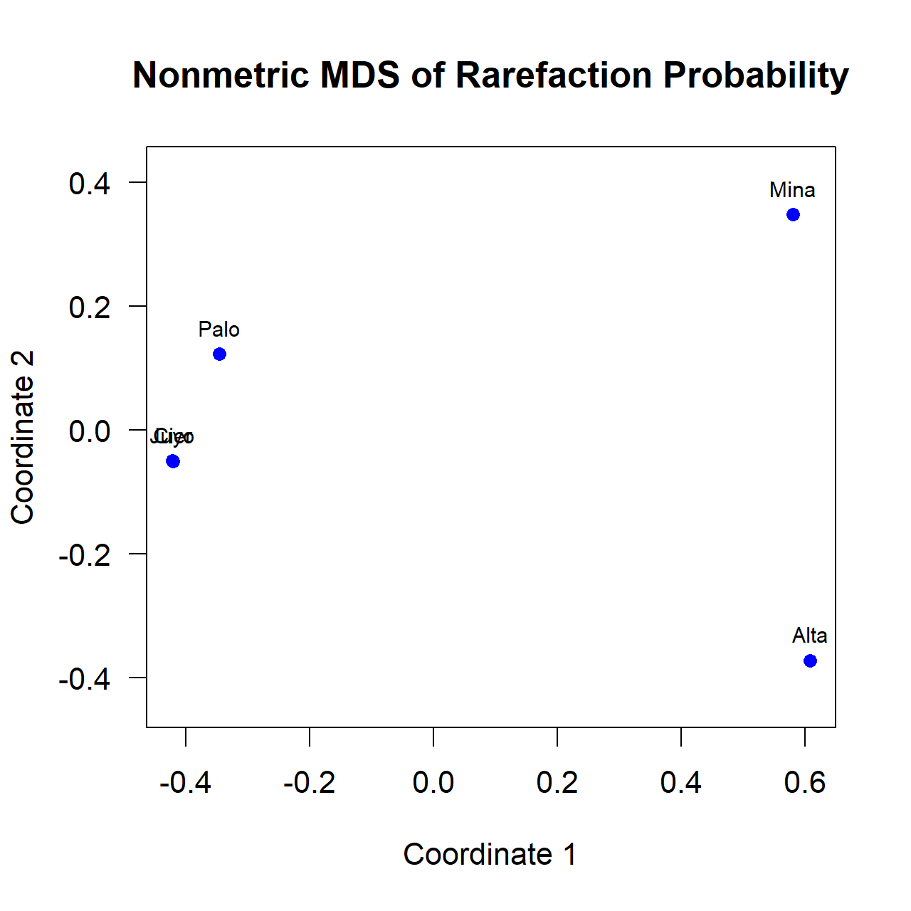
olabel <- scan(filename,what="list", nlines=1) olabel data <- scan(filename,skip=1) #data num_cols <- (1 + sqrt(1 + 8*length(data)))/2 - 1 mat <- matrix(0, num_cols, num_cols) mat[row(mat) <= col(mat)] <- data mat <- t(mat) #mat #Finally to get a 'dist' object: #Probabilities converted to distance with 1-p Rarefaction Trace Plot Output (conkey_p.csv) 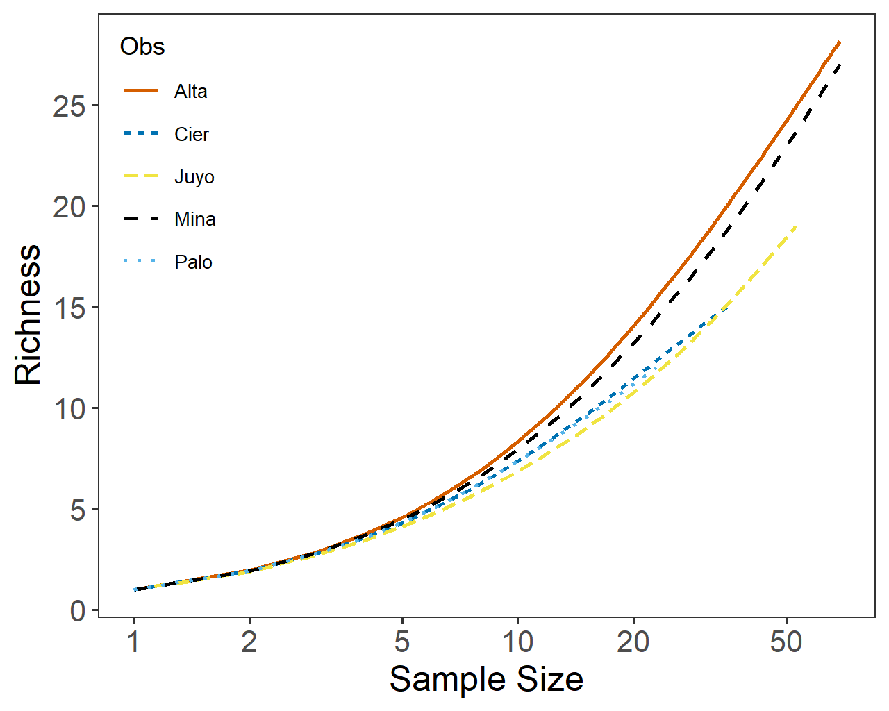
Obs,SS,Richness,Std
"Palo",1,1.00,0.00
"Palo",2,1.93,0.26
"Palo",3,2.79,0.42
...
"Palo",22,11.74,0.44
"Palo",23,12.00,0.00
"Cier",1,1.00,0.00
"Cier",2,1.92,0.26
...
"Cier",35,15.00,0.00
"Juyo",1,1.00,0.00
"Juyo",2,1.90,0.30
...
"Juyo",53,19.00,0.00
"Mina",1,1.00,0.00"Mina",2,1.94,0.23
...
"Mina",69,27.00,0.00
"Alta",1,1.00,0.00
"Alta",2,1.96,0.20
...
"Alta",69,28.16,2.05
The following R code will produce a rarefaction trace from this output file. library("ggplot2")
library("plyr")
library("dplyr")
filename <- "conkey_p.csv"
trace <- read.csv(filename)

cbPalette <- c( "#D55E00","#0072B2", "#F0E442","#000000","#56B4E9",
"#E69F00","#009E73","#CC79A7")

trace <- replace(trace, trace == 0, NA)
trace <- data.frame(trace)

png("conkeyTrace.png",width=5,height=4,units="in",res=256)
ggplot(trace, aes(x=SS, group=Obs, color=Obs, linetype=Obs,)) +
  geom_line(aes(y=Richness), size=0.75) +

# uncommenting this & next lines add +/- SD line for each case
#  geom_line(aes(y=Richness+Std), size=0.75) +
#  geom_line(aes(y=Richness-Std), size=0.75) +

  scale_x_log10(name='Sample Size',
     breaks=c(1,2,5,10,20,50,100,200,500,1000,2000,5000)) +
#use next 2 lines instead of previous 2 for linear X scale
#  scale_x_continuous(name='Sample Size', +
#     limits=c(0,50),breaks=seq(0,50,5)) +

  scale_y_continuous(name='Richness', breaks=seq(0,200,5)) +
  theme_bw() +
  theme(axis.text.x = element_text(size=12),  axis.text.y = element_text(size=12),
        axis.title.x = element_text(size = 14),axis.title.y = element_text(size = 14),
        panel.grid.major = element_blank(), panel.grid.minor = element_blank())+

  theme(legend.position = c(0.01,0.99),
        legend.justification = c(0, 1),
        legend.text=element_text(size=8),
        legend.title=element_text(size=10)) +
  scale_colour_manual(values=cbPalette)
dev.off()
References Cited Baxter, M. J. 2001 Methodological Issues in the Study of Assemblage Diversity. American Antiquity. 66(4): 715-725. |
| Home | Top | Program Overview | Ordering | Documentation | Bibliography |
| Page Updated: 14 February 2026 |