TFQA: Tools for Quantitative Archaeology
kintigh@tfqa.com +1 (505)
395-7979
TFQA Home
TFQA Documentation
TFQA Orders
Kintigh(ASU
Directory)
 |
TFQA: Tools for Quantitative Archaeology |
TFQA Home |
Page TitleKMPLT: Plot k-means Results on Screen and a Plotter
Program KMPLT creates screen and hard-copy graphical plots of the results produced by program KMEANS. (See the section "HARDWARE SUPPORT" under "Program Conventions" above. RUNNING KMPLT You can produce either screen or plotter plots or both, on the same run. Because this program runs very quickly, if you have both a graphics card and a plotter you should preview program results on the screen before plotting them (which takes a little while, because the plotter is slow). To start the program type: KMPLT<Enter> or KMPLT <filename><Enter> where <filename> is a k-means plot file.
SEQUENCE OF KMPLT PROGRAM PROMPTS Kmeans Plot File {.PLT} ? Data File Read: xx/xx/xx - xxxxxxxxxxxxxxxxx Tabulation Variable 3 has been Read
After the program greeting message, you are prompted for the plot output file produced by KMEANS. Enter the file name of that file. The program assumes that the file extension is .PLT, so "FIBULA" and "FIBULA.PLT" have exactly the same effect. (If the plot file name has no extension, e.g. "PLOT", enter a period after the file name: "PLOT.".) The program will respond with the title line and date of that run of the KMEANS program (assuming that the calendar was properly set). If this is incorrect, hit <Ctrl><Break> and start again with the program. If Kmeans was run with a tabulation variable, that variable is reported. Read an Alternate Tabulation Variable {N} ?
If you wish to plot an alternate tabulation variable, the program will prompt for another file name and ask you to select the column of the Antana format file to be used. Plot a File of Reference Lines and Points {N} ?
It is possible to overlay the scatter plots with a sequence of reference lines or points. The format of this file is that used by HPPLOT to plot lines and points. See the HPPLOT documentation for reference.
Plot to HPGL Plotter or HP LaserJet Printer {N} ? HPGL Output to (PRN, COM1, COM2 or <filename>) ? HP [L]aserJet 3/4 or Plotter Paper Size: [A] 8.5x11 [B] 11x17 {L} ?
Enter Y to the first question to produce a hard-copy plot. If Y is entered, the program prompts for the file or device name, either a regular file name, PRN, COM1 or COM2, depending on what port the printer or plotter is connected to. If you're using a HP Laserjet III or above printer reply PRN. If you're going to import the file into Word Perfect or another program, reply with a file name. You then select L for HP laserjet III or above (this does not work for earlier Laserjets) or A or B for the plotter paper size. If you will incorporate the plot into Word Perfect, enter A or B, not L; the paper size does not matter.
[S]SE Plot, Random-Data [D]ifference, or [Q]uit {S} ? Plot: [S]SE, [L]og10(%SSE), or [D]istance: Sqrt(SSE/N) {L} ? Random Run Plot: [A]ll, [M]ean/Std, [N]one {A} ? Do You Want a Pen Plot {Y} ? Prepare Plotter and Hit Return When Ready {Y} ?
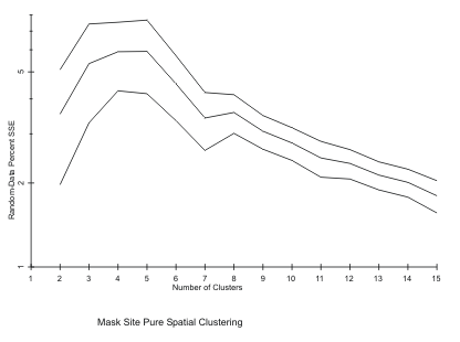
Next, the program will plot the %SSE values. By default, a Log10(SSE) plot by cluster size is produced (Figure 6). Alternately the total SSE can be plotted or a distance-related measure √SSE/N can be plotted (Figure 7; see Gregg et al. 1991). The actual data are plotted with a solid line; random runs are plotted with dotted lines and dashed lines. If you have a plotter, the program will ask if you want a pen and ink plot of the SSE graph. If you do, reply Y to the second plot and press <Enter> when the plotter is loaded with paper. When you have finished viewing this plot, hit <enter>.
X Values Range from 34.94 to 41.66 Xmin {?} ? Xmax {?} ? Y Values Range from 48.08 to 60.79 Ymin {?} ? Ymax {?} ?
The program then tells you the range of actual X values prompts you for the range to plot. Often a better-looking axis label will result if the range is further rounded. The program then prompts for the same information regarding the Y axis.
Axes: Equal [L]ength, Equal [S]cale, [F]it Screen, [U]ser Specified {S} ?
The program asks whether the plotted axes should be equal length (with the specified range for each), and equal scale (a unit difference is the same horizontal or vertical difference--use this for distribution maps), or to fit the screen (scale the axes to the maximum length to fit on the screen).
Clustering Level to Plot (0 to Quit) ?
The program wants to know which cluster configuration you want to see. Reply with the number of clusters you would like to see plotted or hit 0 to finish viewing the cluster configurations. Each point will be plotted against the variables identified as plot variables in the original data set (even if the original data set is standardized, the plot is of unstandardized values). The symbol at each point is the cluster number of that point. Each cluster centroid is plotted with a cross.  Figure 7. Random-Data
Log SSE Difference Figure 7. Random-Data
Log SSE Difference
Plot [R]MS Radius Circles, [P]ie Chart, [N]either {R} ?
Plot Points {Y} ?
If only two variables have been clustered (as in pure locational clustering) and the data have not been standardized the program will ask if you want to see the RMS circles around the centroids. If a tabulation variable has been used, it is possible to get pie charts indicating the composition of the clusters by type with the size of the chart equal to that of an RMS circle. Neither, indicates plot only the points. If you have asked for RMS circles or a pie chart the programs asks if you want also to see the points. Note that the pie charts are not properly imported by Word Perfect (5.0 or 5.1) but will appear with a plotter or direct output to a Laserjet supporting HPGL.
Do You Want a Pen Plot {Y} ? Prepare Plotter and Hit Return When Ready {Y} ?
If you have indicated that you wish to make plotter plots, you will see the first prompt, immediately above, before any of the possible displays are plotted. For each positive response to this prompt, you will see the second prompt.
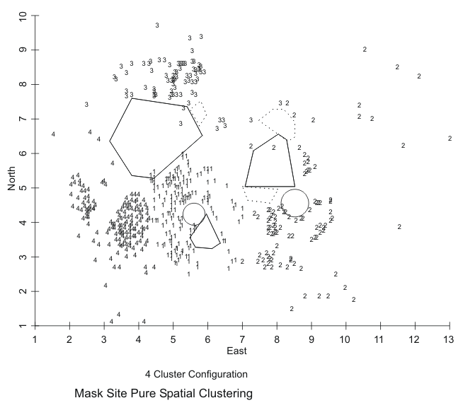
At this point the plot(s) will be produced (Figure 8). Note that one or the other axis may be lengthened to provide proper screen scaling. Hit <Enter> to continue after you have viewed a plot. You will then be asked again what cluster configuration you want to see.
Elapsed Time: 4.29 Minutes End KMEANPLT  Figure 8. KMEANS Pure Spatial Clustering of Mask Site Artifacts, 4 Cluster Solution. Figure 8. KMEANS Pure Spatial Clustering of Mask Site Artifacts, 4 Cluster Solution. |
| Home | Top | Overview | Ordering | Documentation |
| Page Updated: 5 February 2026 |