A Refinement of Rice and Plog's Method of
Estimating Areas Sampled by Trenches
Keith W. Kintigh - May 14, 2007
Rice and Plog present a persuasive argument for the use of mechanical trenching as a sampling strategy for the identification of features that have little or no surface visibility. I suggest a refinement of their argument and formulae for the estimated sampled area (ESA) that allows for the explicit treatment of a broader class of problems.
 Rice
and Plog rather vaguely use the terms "feature width" and
"average feature dimension" in deriving their formulae. However, the
attribute of feature size that is significant from the standpoint of figuring a
sampling fraction for a trenching strategy is the average length of the
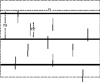
perpendicular exposure of a class of features to the trenches (see
Figure). This can be most easily seen by looking at a simplified model in
which a set of evenly-spaced parallel trenches (of negligible width) overlay a
set of features idealized as lines representing their perpendicular exposures.
If trenches are 10m apart, and the features have an average exposure of 5m
perpendicular to the trenches, then, on the average, 50% of the features will
be located by the trenches. If the average feature exposure was 2m, the sample
fraction drops to 20%. Rice
and Plog rather vaguely use the terms "feature width" and
"average feature dimension" in deriving their formulae. However, the
attribute of feature size that is significant from the standpoint of figuring a
sampling fraction for a trenching strategy is the average length of the
perpendicular exposure of a class of features to the trenches (see
Figure). This can be most easily seen by looking at a simplified model in
which a set of evenly-spaced parallel trenches (of negligible width) overlay a
set of features idealized as lines representing their perpendicular exposures.
If trenches are 10m apart, and the features have an average exposure of 5m
perpendicular to the trenches, then, on the average, 50% of the features will
be located by the trenches. If the average feature exposure was 2m, the sample
fraction drops to 20%.
It
turns out that if the features are randomly located, in general, a trench of
negligible width samples a strip of width FE, where FE is the
average length of a perpendicular exposure of a class of features to the
trench. Assuming the trench spacing (TS) is greater than the feature
exposure, if only one side of a trench of length TL is profiled and
evaluated, for estimation purposes, the trench may be assumed to have
negligible width and the estimated sample area, ESA, is:
1.
ESAFE = FE x TL (analogous to Rice and Plog's
equation 1).
If
both sides of the trench are profiled (and FE >> TW) then a
trench of width, TW, samples an area:
2.
ESAFE = (FE+TW) x TL (analogous to Rice
and Plog's equation 3).
The
sample fraction pFE for a given feature exposure dimension
is simply the total area sampled (TA, including overlapping sampled
areas only once) divided by the estimated sample area.
3.
pFE=ESAFE / TA
The
key point here is that the sample fraction is not a constant but is a function
of the feature exposure. The estimated number of features can be obtained by
dividing the number of features located of a particular size (exposure) class
by the sample fraction for that size class of features.
Thus
in the examples of trenches spaced 10m apart the sample fractions for 5m- and
2m-exposure features (e.g., pithouses and pits) are .5 and .2. If we locate 5
of the 5m features in trenches then the estimated number of features of that
size class is 5/.5=10. If we locate 5 of the 2m exposure features then the
estimated number in the sampled area is 5/.2=25.
The
advantage of this statement over Rice and Plog's formulae is that it allows us
to deal explicitly with other than circular features. The formulae given by
Rice and Plog are only correct where the "width" is of an
"ideal," i.e. circular, feature. They do not state how they obtained
feature widths for non-circular features, notably pithouses.
Clearly,
the length of the perpendicular exposure of a circular feature is simply its
diameter. For randomly oriented rectangular features the length of the
perpendicular exposure is not so obvious, but it is obtained by averaging the
perpendicular exposure of a feature as it is rotated around a circle. For a
rectangular feature of length FL, and width FW, the average
perpendicular exposure is:

By
way of application, it is probably preferable to assume that pithouses are
rectangular rather than circular. At Snaketown, the mean house width is 3.7m
and the mean length is 6.2m (81 19). Substituting in equation 3 (i.e.,
assuming the pithouses are rectangular), we get an average exposure of 6.3m,
which, it may be noted, is longer than the average pithouse length (this effect
is exaggerated the more nearly square a feature becomes).
Once
the key concept of perpendicular exposure is accepted, it is possible to deal
with arbitrary shapes and orientations of features. For simple shapes with
random orientations, calculus will provide a solution to the problem of
determining the average perpendicular exposure. For more complex shapes and
when orientations are non-random, simple computer modeling may be required (see
Abbott 1985). For example, we know that Hohokam pithouses are not randomly
oriented, but at least in some cases show systematic orientations (Wilcox
1981).
References Cited<
Abbott,
David. 1985. Unbiased Estimates of Feature Frequencies with Computer
Simulation. American Archaeology 5(1): 4-11.
Wilcox,
David R., Thomas R. McGuire, and Charles Sternberg. 1981. Snaketown
Revisited: A Partial Cultural Resource Survey, Analysis of Site Structure and
an Ethnohistorical Study of the Proposed Hohokam-Pima National Monument,
Arizona State Museum, Archaeological Series No. 155.
|